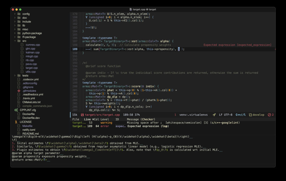

Emacs is my preferred tool for development, statistical computing, and writing. The killer feature is without doubt https://orgmode.org/ which allows for powerful literate programming, handling of bibliographies, organizing notes collections, and much more.
I finally decided to make the move from my vanilla emacs configuration to Doom Emacs. This gives an optimized emacs experience with fast load times due to lazy-loading of packages, and more importantly, the maintainer is doing an amazing job on adapting to new features and changes to emacs and the various lisp packages. A task which I found increasingly time-consuming.

The Cantor ternary set is a remarkable subset of the real numbers
named after German mathematician Georg Cantor who described the set
in 1883. It has the same cardinality as
The set can be constructed recursively by first considering the unit
interval
The recursion can be illustrated in python in the following way
  import numpy as np

  def transform_interval(x, scale=1.0, translation=0.0):
      return tuple(map(lambda z: z * scale + translation, x))

  def Cantor(n):
      if n==0: return {(0,1)}
      Cleft = set(map(lambda x: transform_interval(x, scale=1/3), Cantor(n-1)))
      Cright = set(map(lambda x: transform_interval(x, translation=2/3), Cleft))
      return Cleft.union(Cright)
ML-inference in non-linear SEMs is complex. Computational intensive methods based on numerical integration are needed and results are sensitive to distributional assumptions.
In a recent paper: A two-stage estimation procedure for non-linear structural equation models by Klaus Kähler Holst & Esben Budtz-Jørgensen (https://doi.org/10.1093/biostatistics/kxy082), we consider two-stage estimators as a computationally simple alternative to MLE. Here both steps are based on linear models: first we predict the non-linear terms and then these are related to latent outcomes in the second step.


Logic gates are the building blocks of digital electronics. Simple logic gates are efficiently implemented in various IC packages such as the 74HCXX series. However, it is educational to have a look at the implementation using just NPN transistors.
A small illustration on using the
armadillo C++ linear algebra
library for solving an ordinary differential equation of the form
The abstract super class Solver
defines the methods solve (for approximating the solution in
user-defined time-points) and solveint (for interpolating user-defined
input functions on finer grid). As an illustration a simple
Runge-Kutta solver is derived in the class RK4.
The first step is to define the ODE, here a simple one-dimensional ODE
rowvec dX(const rowvec &input, // time (first element) and additional input variables
	 const rowvec &x,     // state variables
	 const rowvec &theta) {   // parameters
  rowvec res = { theta(0)*theta(1)*(input(1)-x(0)) };
  return( res );
}
The ODE may then be solved using the following syntax
odesolver::RK4 MyODE(dX);
arma::mat res = MyODE.solve(input, init, theta);
with the step size defined implicitly by input (first column is the time variable
and the following columns the optional different input variables) and
boundary conditions defined by init.
Assume that two positive numbers are given,
A player draws randomly one of the numbers and has to guess if the
number is smaller or larger than the other unrevealed number, i.e.,
let
A random guess (coin-flip) would due to the sampling
The 74HC595: an 8-bit serial-in/serial or parallel-out shift register with a storage register and 3-state outputs.
If higher load is required there is also the TPIC6C595 (e.g., for driving LEDs), or it should be paired with for example ULN2803 or similar. For multiple inputs see the 74HC165.

The basic usage is to serially transfer a byte from a microcontroller to the IC. When latched the byte will then in parallel be available on output pins QA-QH (Q0-Q7).
Let
Let