Doubly Robust

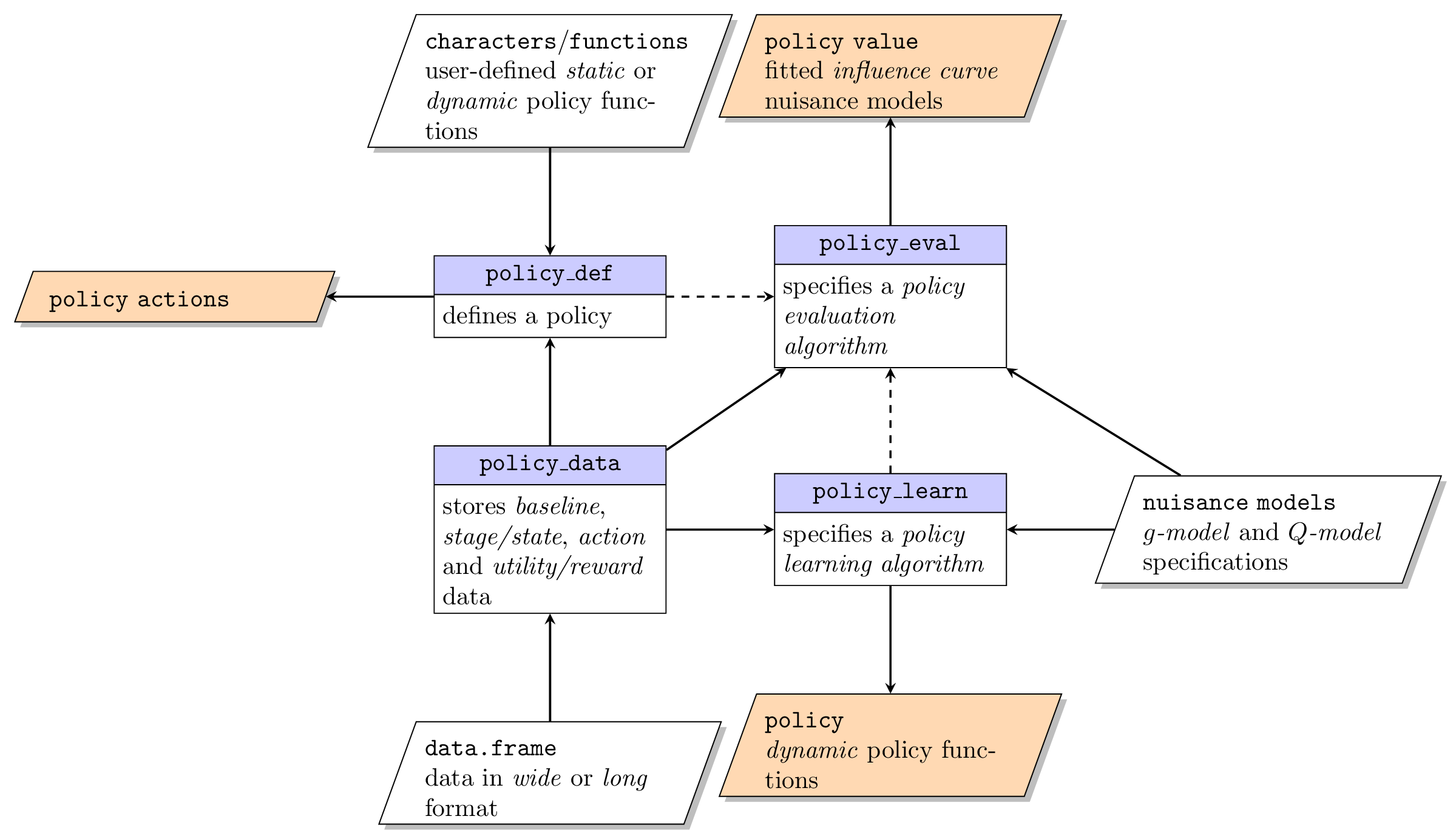
The R package polle is a unifying framework for learning and evaluating finite stage policies based on observational data. The package implements a collection of existing and novel methods for causal policy learning including doubly robust restricted Q-learning, policy tree learning, and outcome weighted learning. The package deals with (near) positivity violations by only considering realistic policies. Highly flexible machine learning methods can be used to estimate the nuisance components and valid inference for the policy value is ensured via cross-fitting. The library is built up around a simple syntax with four main functions policy_data(), policy_def(), policy_learn(), and policy_eval() used to specify the data structure, define user-specified policies, specify policy learning methods and evaluate (learned) policies. The functionality of the package is illustrated via extensive reproducible examples.

\[ \newcommand{\pr}{\mathbb{P}}\newcommand{\E}{\mathbb{E}} \] Relative risks (and risk differences) are collapsible and generally considered easier to interpret than odds-ratios. In a recent publication Richardson et al (JASA, 2017) proposed a new regression model for a binary exposure which solves the computational problems that are associated with using for example binomial regression with a log-link function (or identify link for the risk difference) to obtain such parameter estimates. Let \(Y\) be the binary response, \(A\) binary exposure, and \(V\) a vector of covariates, then the target parameter is \begin{align*} &\mathrm{RR}(v) = \frac{\pr(Y=1\mid A=1, V=v)}{\pr(Y=1\mid A=0, V=v)}. \end{align*} Let \(p_a(V) = \pr(Y \mid A=a, V), a\in\{0,1\}\), the idea is then to posit a linear model for \[ \theta(v) = \log \big(RR(v)\big) \] and a nuisance model for the odds-product \[ \phi(v) = \log\left(\frac{p_{0}(v)p_{1}(v)}{(1-p_{0}(v))(1-p_{1}(v))}\right) \] noting that these two parameters are variation independent which can be from the below L’Abbé plot. Similarly, a model can be constructed for the risk-difference on the following scale \[\theta(v) = \mathrm{arctanh} \big(RD(v)\big).\] ...